Getting Started 3: Classic Machine Learning for Cybersecurity


In this tutorial, we will use basic machine learning algorithms to gain insights into network traffic and detect potential cyber attacks.
Tutorial Objectives
By the end of this tutorial, you will be able to:
Preprocess and clean data for machine learning.
Extract meaningful features from raw data to use in machine learning models.
Train a machine learning model using scikit-learn.
Evaluate the performance of your model using appropriate metrics.
[32]:
### Importing required libraries

import numpy as np
import matplotlib.pyplot as plt

from sklearn import datasets
from sklearn.model_selection import train_test_split
from sklearn.metrics import confusion_matrix
from sklearn.decomposition import PCA
from sklearn.preprocessing import StandardScaler, OneHotEncoder
from sklearn.metrics import confusion_matrix, ConfusionMatrixDisplay, classification_report
from sklearn.cluster import KMeans, DBSCAN
from sklearn.linear_model import LogisticRegression
from sklearn.naive_bayes import GaussianNB
from sklearn.svm import SVC
Data Preprocessing
In this section, we will work with the KDD Cup 99 dataset, a widely used benchmark for evaluating network intrusion detection algorithms. This dataset contains simulated network traffic, including both normal connections and a small fraction of attack events.
The dataset contains a mix of continuous and categorical features describing TCP connections, login attempts, and traffic patterns. Key feature categories include:
Basic connection features – e.g.,
duration,protocol_type,service,src_bytes,dst_bytes,flag,land,wrong_fragment,urgent.Content features – e.g.,
hot,num_failed_logins,logged_in,num_compromised,root_shell,su_attempted.Traffic features over a 2-second time window – e.g.,
count,srv_count,serror_rate,srv_serror_rate,rerror_rate,srv_rerror_rate.
Load and Process the KDDCUP99 Dataset
We’ll use the SA subset of the data to keep computation manageable. It contains mostly normal connections with a small fraction of attacks (~1–3%).
[33]:
# Load KDDCup99 dataset (subset for demonstration)
X, y = datasets.fetch_kddcup99(
    subset="SA",             # Use the 'SA' subset (smaller sample)
    percent10=True,          # Use 10% of the full dataset for efficiency
    random_state=42,         # Ensure reproducibility
    return_X_y=True,         # Return data and labels separately
    as_frame=True            # Load as pandas DataFrame
)

# Convert binary label: 1 = attack, 0 = normal
y = (y != b"normal.").astype(np.int32)

n_samples, anomaly_frac = X.shape[0], y.mean()
print(f"{n_samples} datapoints with {y.sum()} anomalies ({anomaly_frac:.02%})")
100655 datapoints with 3377 anomalies (3.36%)
We convert labels and predictions into binary format:
0→ Normal1→ Anomaly
The SA dataset contains 41 features out of which 3 are categorical: protocol_type, service and flag. We will explicitly convert these columns to the category data type and ensure that all other features are treated as numeric.
[34]:
# Ensure categorical columns are 'category'
cat_columns = ["protocol_type", "service", "flag"]
X[cat_columns] = X[cat_columns].astype("category")

# Ensure numeric columns are float
numeric_features = X.columns.difference(cat_columns)  # all other columns
X[numeric_features] = X[numeric_features].astype(float)

# Update categorical features in case dtype changed
categorical_features = X.select_dtypes(include=["category"]).columns
numeric_features = X.select_dtypes(include=["number"]).columns
OneHotEncoder from sklearn.preprocessing.StandardScaler to have zero mean and unit variance. Finally, the processed numeric and categorical features are combined into a single array suitable for model training.[35]:
# One-hot encode categorical features
encoder = OneHotEncoder(sparse_output=False, handle_unknown="ignore")
X_cat = encoder.fit_transform(X[categorical_features])

# Standardize numeric features
scaler = StandardScaler()
X_num = scaler.fit_transform(X[numeric_features])

# Combine processed numeric and categorical features
X_processed = np.hstack([X_num, X_cat])
We split the dataset into training (80%) and testing (20%) subsets.
[36]:
# Split into training and test sets
X_train, X_test, y_train, y_test = train_test_split(
    X_processed, y, test_size=0.2, random_state=42, stratify=y
)

# Print dataset sizes
print("Training samples:", len(X_train))
print("Testing samples:", len(X_test))
Training samples: 80524
Testing samples: 20131
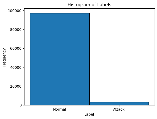
Visualize the distribution of Normal vs Attack labels in the dataset to understand the balance between normal connections and attacks.
[37]:
# Plot label distribution
plt.hist(y, bins=[-0.5, 0.5, 1.5], edgecolor='black')
plt.xticks([0, 1], ['Normal', 'Attack'])
plt.title('Histogram of Labels')
plt.xlabel('Label')
plt.ylabel('Frequency')
plt.show()
Notes:
fetch_kddcup99()conveniently downloads and loads the dataset from scikit-learn’s built-in datasets.Labels are converted from text (
b"normal.",b"attack") to integers (0and1).The histogram provides a quick look at class imbalance, which is typical in cybersecurity data — attacks are rarer than normal events.
Using only 10% of the dataset keeps the demo lightweight while preserving statistical patterns.
Unsupervised Learning with the KDDCUP99 Dataset
Unsupervised learning methods allow us to detect patterns and clusters in the network traffic dataset without using labels. In this section, we demonstrate K-Means, DBSCAN, and Hierarchical Clustering on PCA-reduced KDDCUP99 data.
PCA (Principal Component Analysis)
[38]:
# Reduce dimensionality for visualization
pca = PCA(n_components=8)
X_pca = pca.fit_transform(X_processed)
Notes:
PCA maximizes the variance captured in the reduced space.
Principal components are uncorrelated (orthogonal).
Often used for visualization, noise reduction, and improving clustering efficiency.
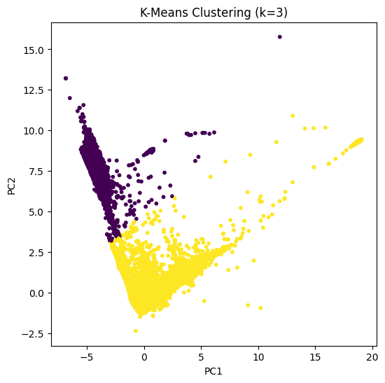
K-Means Clustering
Mathematical Idea: K-Means partitions \(n\) points \(\{x_1, ..., x_n\}\) into \(k\) clusters \(C_1,...,C_k\) by minimizing:
\(J = \sum_{i=1}^{k} \sum_{x \in C_i} \|x - \mu_i\|^2\)
where \(\mu_i\) is the centroid of cluster \(C_i\).
[39]:
# K-Means with 2 clusters
kmeans = KMeans(n_clusters=2, random_state=42)
kmeans_labels = kmeans.fit_predict(X_pca)

# Plot K-Means clusters
plt.figure(figsize=(6,6))
plt.scatter(X_pca[:, 0], X_pca[:, 1], c=kmeans_labels, cmap='viridis', s=10)
plt.title("K-Means Clustering (k=2)")
plt.xlabel("PC1")
plt.ylabel("PC2")
plt.show()
Notes:
K-Means partitions data into \(k\) clusters based on similarity.
Each point is assigned to the nearest cluster centroid.
Requires specifying the number of clusters \(k\) which is often done using the Elbow Method.
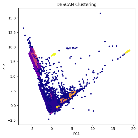
DBSCAN – Density-Based Spatial Clustering
DBSCAN is a non-parametric clustering algorithm which clusters points based on density:
A point is a core point if at least
min_samplespoints are withinepsdistance.Border points are reachable from core points.
Noise points are those not reachable from any core point.
[40]:
# DBSCAN clustering
dbscan = DBSCAN(eps=0.5, min_samples=25)
dbscan_labels = dbscan.fit_predict(X_pca)

# Plot DBSCAN clusters
plt.figure(figsize=(6,6))
plt.scatter(X_pca[:, 0], X_pca[:, 1], c=dbscan_labels, cmap='plasma', s=10)
plt.title("DBSCAN Clustering")
plt.xlabel("PC1")
plt.ylabel("PC2")
plt.show()
Notes:
DBSCAN groups points based on density.
Can detect outliers as points not belonging to any cluster (label = -1).
Does not require specifying the number of clusters (non-parametric).
Supervised Learning with the KDDCUP99 Dataset
In this section, we will demonstrate classic supervised learning algorithms that require labeled data, specifically Logistic Regression and Naive Bayes, to detect attacks in network traffic.
Logistic Regression
Logistic Regression is a classic supervised learning algorithm used for binary classification tasks.
Mathematical Idea:
Logistic Regression models the probability that a given input belongs to a class using the logistic (sigmoid) function:
\(P(y=1 \mid \mathbf{x}) = \sigma(\mathbf{w}^\top \mathbf{x} + b) = \frac{1}{1 + \exp(-(\mathbf{w}^\top \mathbf{x} + b))}\)
where:
\(\mathbf{x}\) is the feature vector,
\(\mathbf{w}\) are the model weights,
\(b\) is the bias term,
\(\sigma(\cdot)\) is the sigmoid function mapping any real number to \([0,1]\).
The model is trained by minimizing the binary cross-entropy loss:
\(\mathcal{L} = -\frac{1}{N} \sum_{i=1}^{N} \left[ y_i \log \hat{y}_i + (1-y_i) \log (1-\hat{y}_i) \right]\)
where \(\hat{y}_i = P(y=1 \mid \mathbf{x}_i)\) and \(y_i \in \{0,1\}\).
[41]:
# Train logistic regression
lr = LogisticRegression(max_iter=1000, random_state=42)
lr.fit(X_train, y_train)

# Predictions
y_pred_lr = lr.predict(X_test)

# Confusion matrix
cm_lr = confusion_matrix(y_test, y_pred_lr)
disp_lr = ConfusionMatrixDisplay(confusion_matrix=cm_lr, display_labels=["Normal", "Attack"])
disp_lr.plot(cmap="Blues")
plt.title("Confusion Matrix – Logistic Regression")
plt.show()

# Classification report
print(classification_report(y_test, y_pred_lr, target_names=["Normal", "Attack"]))
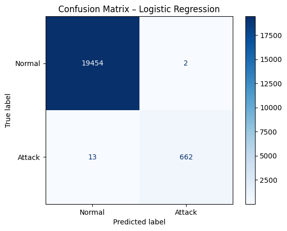
              precision    recall  f1-score   support

      Normal       1.00      1.00      1.00     19456
      Attack       1.00      0.98      0.99       675

    accuracy                           1.00     20131
   macro avg       1.00      0.99      0.99     20131
weighted avg       1.00      1.00      1.00     20131
Notes:
Logistic Regression models the probability of class membership using a linear combination of features.
Suitable for binary classification problems like normal vs attack detection.
Standardizing features improves convergence and performance.
Gaussian Naive Bayes
Gaussian Naive Bayes is a classic supervised learning algorithm based on Bayes’ theorem and the assumption that features are conditionally independent given the class label.
Mathematical Idea:
For a feature vector \(\mathbf{x} = [x_1, x_2, \dots, x_d]\) and a class \(y \in \{0,1\}\), Gaussian Naive Bayes models the class conditional probability as:
\(P(\mathbf{x} \mid y) = \prod_{j=1}^{d} P(x_j \mid y)\)
Assuming each feature \(x_j\) follows a Gaussian distribution for class \(y\):
\(P(x_j \mid y) = \frac{1}{\sqrt{2 \pi \sigma_{y,j}^2}}\exp\left(-\frac{(x_j - \mu_{y,j})^2}{2 \sigma_{y,j}^2}\right)\)
where:
\(\mu_{y,j}\) is the mean of feature \(x_j\) for class \(y\),
\(\sigma_{y,j}^2\) is the variance of feature \(x_j\) for class \(y\).
The predicted class \(\hat{y}\) is obtained using Bayes’ theorem:
\(\hat{y} = \arg\max_y P(y) \prod_{j=1}^{d} P(x_j \mid y)\)
Gaussian Naive Bayes is particularly fast and works well for high-dimensional numeric data.
[42]:
# Train Gaussian Naive Bayes
gnb = GaussianNB()
gnb.fit(X_train, y_train)

# Predictions
y_pred_gnb = gnb.predict(X_test)

# Confusion matrix
cm_gnb = confusion_matrix(y_test, y_pred_gnb)
disp_gnb = ConfusionMatrixDisplay(confusion_matrix=cm_gnb, display_labels=["Normal", "Attack"])
disp_gnb.plot(cmap="Greens")
plt.title("Confusion Matrix – Gaussian Naive Bayes")
plt.show()

# Classification report
print(classification_report(y_test, y_pred_gnb, target_names=["Normal", "Attack"]))
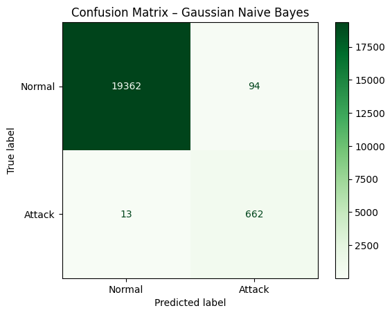
              precision    recall  f1-score   support

      Normal       1.00      1.00      1.00     19456
      Attack       0.88      0.98      0.93       675

    accuracy                           0.99     20131
   macro avg       0.94      0.99      0.96     20131
weighted avg       1.00      0.99      0.99     20131
Notes:
Naive Bayes assumes feature independence given the class label.
GaussianNB models numeric features as normally distributed.
Fast to train and often performs well on high-dimensional datasets.
Support Vector Machine (SVM)
Support Vector Machine (SVM) aims to find the optimal hyperplane that best separates the data into different classes.
Mathematical Idea:
Given a labeled dataset \((x_i, y_i)\), where \(x_i \in \mathbb{R}^n\) and \(y_i \in \{-1, +1\}\), the SVM optimization problem is formulated as:
\(\min_{w, b} \ \frac{1}{2} \|w\|^2\)
subject to:
\(y_i (w \cdot x_i + b) \ge 1, \quad \forall i\)
Here:
\(w\) is the weight vector perpendicular to the separating hyperplane.
\(b\) is the bias term that shifts the hyperplane.
The decision boundary is given by \(w \cdot x + b = 0\).
For non-linearly separable data, SVM uses the kernel trick to implicitly map input features into a higher-dimensional space where a linear separation becomes possible.
Common kernels include:
Linear kernel: \(K(x, x') = x \cdot x'\)
Polynomial kernel: \(K(x, x') = (x \cdot x' + c)^d\)
RBF (Gaussian) kernel: \(K(x, x') = \exp(-\gamma \|x - x'\|^2)\)
The predicted class \(\hat{y}\) for a test point \(x\) is given by:
\(\hat{y} = \text{sign}(w \cdot x + b)\)
SVMs are robust to high-dimensional spaces and effective when the number of features exceeds the number of samples.
[43]:
# Train SVM with RBF kernel
svm_clf = SVC(kernel="rbf", C=1.0, gamma="scale")
svm_clf.fit(X_train, y_train)

# Predictions
y_pred_svm = svm_clf.predict(X_test)

# Confusion matrix
cm_svm = confusion_matrix(y_test, y_pred_svm)
disp_svm = ConfusionMatrixDisplay(confusion_matrix=cm_svm, display_labels=["Normal", "Attack"])
disp_svm.plot(cmap="Blues")
plt.title("Confusion Matrix – Support Vector Machine (RBF Kernel)")
plt.show()

# Classification report
print(classification_report(y_test, y_pred_svm, target_names=["Normal", "Attack"]))
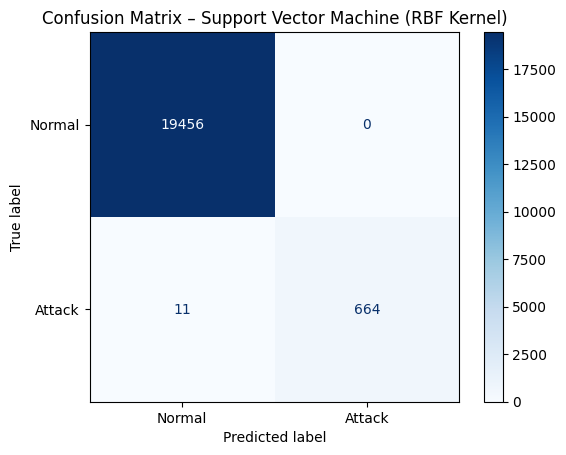
              precision    recall  f1-score   support

      Normal       1.00      1.00      1.00     19456
      Attack       1.00      0.98      0.99       675

    accuracy                           1.00     20131
   macro avg       1.00      0.99      1.00     20131
weighted avg       1.00      1.00      1.00     20131
Notes:
SVMs aim to maximize the margin between classes for better generalization.
The RBF kernel is often effective for non-linear relationships.
Parameter tuning (e.g.,
Candgamma) can significantly impact performance.SVMs work well in high-dimensional spaces, but training can be computationally intensive on very large datasets.
Exercises
In this exercise, we’ll learn how to fit a Decision Tree classifier and how to evaluate the most important features in the KDD Cup 99 dataset.
Exercise 1: Train Decision Tree Classifier
Train a
DecisionTreeClassifierfromsklearn.treeon the training data. You can find the technikal reference here: DecisionTreeClassifierSet
max_depth=10for a manageable tree size.Train the model with the allready imported and scaled data.
Evaluate on the test set using a confusion_matrix.
[44]:
# TODO: Step 1 - Train Decision Tree
# TODO: Step 2 - Predict test labels
# TODO: Step 3 - Print a confusion_matrix
Exercise 2: Visualize the Decision Tree
Use
plot_treefromsklearn.treeto visualize the tree. You can find the reference here: plot_treeLimit depth to 3 for better readability.
Include feature names and class names.
[45]:
# TODO: Step 1 - Visualize Decision Tree
# TODO: Step 2 - Configure plot_tree
# TODO: Step 3 - Show the plot
Exercise 3: Feature Importance
Extract feature importances from the
feature_importances_atttribut in the trained Decision Tree.Plot the top 10 features in a bar chart.
Interpret which features are most indicative of attacks and why.
[46]:
# TODO: Step 1 - Get feature importances
# TODO: Step 2 - Plot top 10 features
# TODO: Step 3 - Interpret results
Exercise 4: Parameter Optimization for SVM
In the SVM example above, we initially guessed the hyperparameters C, gamma, and kernel based on experience. In this exercise, we’ll try to find better parameters using GridSearchCV, which performs cross-validated grid-search over a parameter grid using the estimator’s fit and score methods.
Familiarize yourself with GridSearchCV on the scikit-learn documentation.
Use the provided SVM model and perform a GridSearchCV to tune hyperparameters
C,gamma, andkernel.Identify and print the best parameter combination and cross-validation accuracy from the grid search.
Re-train the SVM using these optimal parameters and evaluate it on the test dataset.
Compare the performance (e.g., accuracy, precision, recall) of the optimized model to the default SVM.
Discuss how parameter tuning affects the margin width, model capacity, and generalization ability of SVMs.
[47]:
# TODO: Step 0 - Import necessary libraries
# TODO: Step 1 - Define the parameter grid for SVM
# TODO: Step 2 - Initialize the SVM classifier
# TODO: Step 3 - Create a GridSearchCV object with 5-fold cross-validation
# TODO: Step 4 - Fit the GridSearchCV on the training data
# TODO: Step 5 - Print the best parameters and best cross-validation score
# TODO: Step 6 - Retrieve the best model and make predictions on the test set
# TODO: Step 7 - Plot the confusion matrix for the best SVM model
# TODO: Step 8 - Print the classification report
# TODO: Step 9 - Interpret results
# - Compare default vs optimized model performance.
# - Discuss how tuning C, gamma, and kernel affected accuracy and generalization.
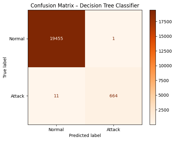
Solution - Exercise 1: Train Decision Tree Classifier
DecisionTreeClassifier from sklearn.tree on the training data (see the technical reference here) and set max_depth=10 for a manageable tree size, using the already imported and scaled data.[48]:
# TODO: Step 1 - Train Decision Tree
from sklearn.tree import DecisionTreeClassifier
dt_clf = DecisionTreeClassifier(max_depth=10, random_state=42)
dt_clf.fit(X_train, y_train)

# TODO: Step 2 - Predict test labels
y_pred = dt_clf.predict(X_test)

# TODO: Step 3 - Print a confusion_matrix
cm = confusion_matrix(y_test, y_pred)
disp = ConfusionMatrixDisplay(confusion_matrix=cm, display_labels=["Normal", "Attack"])
disp.plot(cmap="Oranges")
plt.title("Confusion Matrix – Decision Tree Classifier")
plt.show()
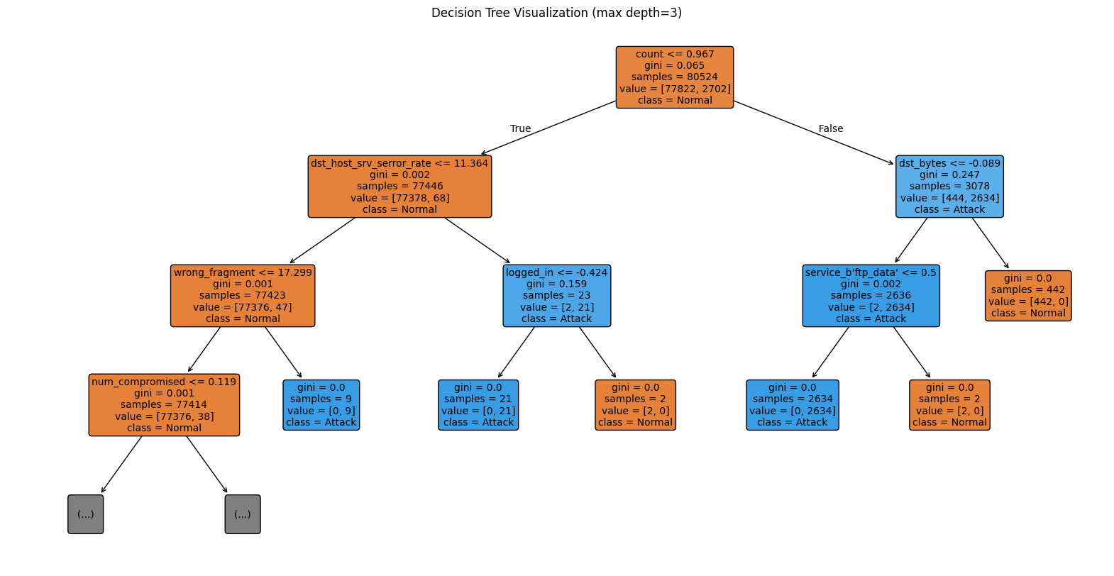
Solution - Exercise 2: Visualize the Decision Tree
plot_tree from sklearn.tree to visualize the decision tree (see the reference here) and limit the depth to 3 for better readability.[49]:
# TODO: Step 1 - Visualize Decision Tree
from sklearn.tree import plot_tree
plt.figure(figsize=(20,10))

# TODO: Step 2 - Configure plot_tree
plot_tree(dt_clf, max_depth=3, feature_names=list(numeric_features) + list(encoder.get_feature_names_out(categorical_features)),
          class_names=["Normal", "Attack"], filled=True, rounded=True, fontsize=10)

# TODO: Step 3 - Show the plot
plt.title("Decision Tree Visualization (max depth=3)")
plt.show()
Solution - Exercise 3: Feature Importance
feature_importances_ attribute of the trained Decision Tree and plot the top 10 features in a bar chart.[50]:
import seaborn as sns
# TODO: Step 1 - Get feature importances
importances = dt_clf.feature_importances_
indices = np.argsort(importances)[::-1]
feature_names = list(numeric_features) + list(encoder.get_feature_names_out(categorical_features))
# TODO: Step 2 - Plot top 10 features
n_top_features = 10
top_n_features = np.array(feature_names)[indices][:n_top_features]
top_n_importances = importances[indices][:n_top_features]

# TODO: Step 3 - Interpret results
plt.figure(figsize=(12, 6))
sns.barplot(x=top_n_importances, y=top_n_features, palette="viridis")
plt.title("Top 10 Feature Importances - Decision Tree")
plt.xlabel("Feature Importance")
plt.ylabel("Feature Name")
plt.show()
/var/folders/zm/0r1v0fg50w53tw219k1jp0ym0000gn/T/ipykernel_39233/4014255988.py:13: FutureWarning:

Passing `palette` without assigning `hue` is deprecated and will be removed in v0.14.0. Assign the `y` variable to `hue` and set `legend=False` for the same effect.

  sns.barplot(x=top_n_importances, y=top_n_features, palette="viridis")
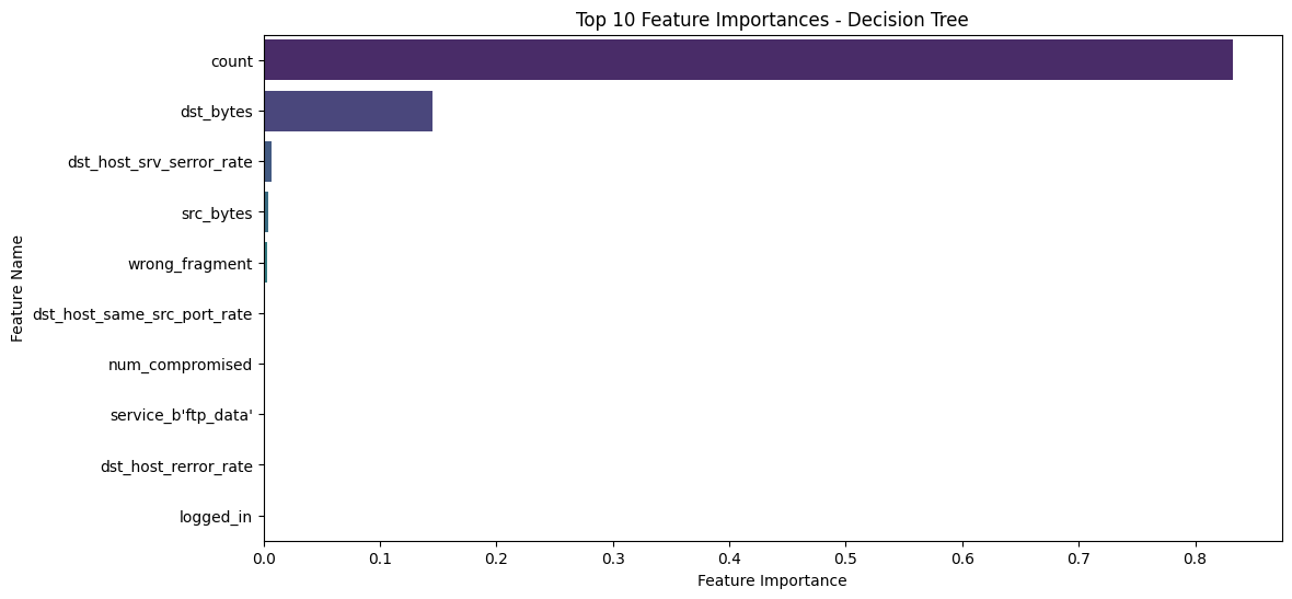
count feature is by far the most important, and the entire classification relies heavily on it. This can pose a problem for the robustness of the classifier if it depends primarily on a single feature. The count feature represents the number of connections to the same host as the current connection in the past two seconds.count, mitigates overfitting, and generally improves the stability and generalization of the classifier.[51]:
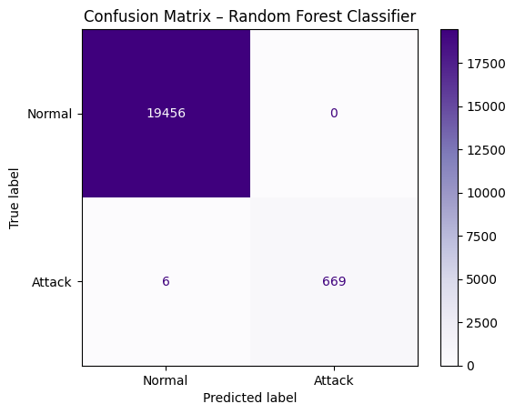
# step 1: implement Random Forest Classifier
from sklearn.ensemble import RandomForestClassifier
rf_clf = RandomForestClassifier(n_estimators=100, max_depth=10, random_state=42)
rf_clf.fit(X_train, y_train)
# step 2 : predict test labels
y_pred_rf = rf_clf.predict(X_test)
#step 3: print confusion matrix
cm_rf = confusion_matrix(y_test, y_pred_rf)
disp_rf = ConfusionMatrixDisplay(confusion_matrix=cm_rf, display_labels=["Normal", "Attack"])
disp_rf.plot(cmap="Purples")
plt.title("Confusion Matrix – Random Forest Classifier")
plt.show()
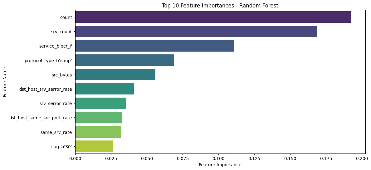
[52]:
# Step 1 - Get feature importances
importances = rf_clf.feature_importances_
indices = np.argsort(importances)[::-1]
feature_names = list(numeric_features) + list(encoder.get_feature_names_out(categorical_features))

# Step 2 - Select top 10 features
n_top_features = 10
top_n_features = np.array(feature_names)[indices][:n_top_features]
top_n_importances = importances[indices][:n_top_features]

# Step 3 - Plot top 10 feature importances
plt.figure(figsize=(12, 6))
sns.barplot(x=top_n_importances, y=top_n_features, palette="viridis")
plt.title("Top 10 Feature Importances - Random Forest")
plt.xlabel("Feature Importance")
plt.ylabel("Feature Name")
plt.show()
/var/folders/zm/0r1v0fg50w53tw219k1jp0ym0000gn/T/ipykernel_39233/3226767616.py:13: FutureWarning:

Passing `palette` without assigning `hue` is deprecated and will be removed in v0.14.0. Assign the `y` variable to `hue` and set `legend=False` for the same effect.

  sns.barplot(x=top_n_importances, y=top_n_features, palette="viridis")
Solution - Exercise 4: Parameter Optimization for SVM
C, gamma, and kernel based on experience.GridSearchCV to systematically search for the best hyperparameter combination, re-train the SVM with these optimal values, and evaluate its performance on the test dataset to analyze the effect on margin width, model capacity, and generalization.[ ]:
# TODO: Step 0 - Import necessary libraries
from sklearn.model_selection import GridSearchCV

# TODO: Step 1 - Define the parameter grid for SVM
# populate grid for better coverage of parameter space
param_grid = {
    'C': [0.1, 10],
    'gamma': ['scale', 'auto'],
    'kernel': ['rbf', 'linear']
}

# TODO: Step 2 - Initialize the SVM classifier
svm_clf = SVC()

# TODO: Step 3 - Create a GridSearchCV object with 5-fold cross-validation
# for debugging and understanding set verbose=2, for the rendering to html it was set to 0
grid_search = GridSearchCV(estimator=svm_clf, param_grid=param_grid,
                           scoring='balanced_accuracy', cv=5, n_jobs=-1, verbose=0) # Use balanced_accuracy for imbalanced data

# TODO: Step 4 - Fit the GridSearchCV on the training data
grid_search.fit(X_train, y_train)

# TODO: Step 5 - Print the best parameters and best cross-validation score
print("Best Parameters:", grid_search.best_params_)
print("Best balanced_accuracy Score:", grid_search.best_score_)

# TODO: Step 6 - Retrieve the best model and make predictions on the test set
best_svm_clf = grid_search.best_estimator_
y_pred_svm = best_svm_clf.predict(X_test)

# TODO: Step 7 - Plot the confusion matrix for the best SVM model
cm_svm = confusion_matrix(y_test, y_pred_svm)
disp_svm = ConfusionMatrixDisplay(confusion_matrix=cm_svm, display_labels=["Normal", "Attack"])
disp_svm.plot(cmap="Blues")
plt.title("Confusion Matrix – Optimized Support Vector Machine")
plt.show()

# TODO: Step 8 - Print the classification report
print("Classification Report:")
print(classification_report(y_test, y_pred_svm))

# TODO: Step 9 - Interpret results
# - Compare default vs optimized model performance.
# - Discuss how tuning C, gamma, and kernel affected accuracy and generalization.
Best Parameters: {'C': 10, 'gamma': 'auto', 'kernel': 'rbf'}
Best Cross-Validation Accuracy: 0.9979521670185185

Classification Report:
              precision    recall  f1-score   support

           0       1.00      1.00      1.00     19456
           1       1.00      0.99      1.00       675

    accuracy                           1.00     20131
   macro avg       1.00      1.00      1.00     20131
weighted avg       1.00      1.00      1.00     20131
Conclusion
In this tutorial, we applied classic machine learning techniques using scikit-learn to cybersecurity tasks, such as detecting network attacks. By preprocessing data, encoding features, and training models, we gained insights into how to effectively classify normal and malicious traffic and how to identify patterns in network data to provide actionable insights for cybersecurity.
 If you found this tutorial helpful, please ⭐ star our repository to show your support.
 For any questions, typos, or bugs, kindly open an issue on GitHub — we appreciate your feedback!